Analysis of Sensing Modalities of Wire Arc Additive Manufacturing

The Additive Manufacturing Team was responsible for interacting with the current WAAM setup inside the MILL by identifying and implementing sensing modalities that could monitor and lead to better control of the WAAM process. Specifically, the central interest focused on obtaining thermal signatures of the system to understand heat dissipation and thermal effects on microstructure. Additionally, the AM team was directed to integrate one process modification to study the effect of cooling or mechanical stimuli on the microstructure of the completed parts. The main task of the AM team was to find connections between control and modified samples via analyzation of FLIR data and microstructure.

Implementation of IR camera in RPI Weld cell

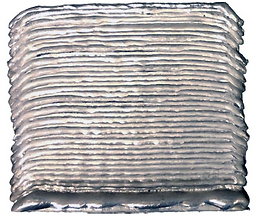
Fan Cooled (FHC) → taller, thinner, less uniform and smooth layers, sharper edges

Still Image from 5 second ILC Workpiece Video

Still Cooled (NHC) → shorter,
thicker, more uniform layers

The increased height of the FHC wall is a result of the cooled temperature of the previous layer- the layer is cooler, so less material is allowed to flow down the sides, as is observed in the NHC (still cooled) piece which is not subject to turbulent flow. Additionally, the sides of the FHC piece were a lot more bulbous and uneven than those in the NHC piece, which is a result of the non-uniform heat distribution from the fan across the part as a function of the distance
between the fan and point of interest on the part. Metallography was performed on both of these samples to compare the grain sizes as a function of build height in the FHC and NHC samples.

As seen in Graphs 2.3.1 and 2.3.2, both temperature profiles demonstrate each weld pass forming a layer with the temperature peaking initially when the weld starts then returning to some steady state value. Both profiles mimic the welding process sufficiently as new layers are welded on top of one another those initial layers are reheated but gradually in more insignificant amounts with more layers in between. Evidently, the highest temperature peak recorded was of the NHC run because the workpiece overall remained at a higher temperature. The box fan did have an overall effect on cooling the FHC workpiece to a lower steady state temperature value relative to the NHC workpiece. Using Graph 2.3.2 as a reference, even when the FHC workpiece had initial welding temperatures higher than that of the NHC one, the box fan more effectively cooled down the workpiece as the weld continued.

Analyzing the cooling rate profiles in Graphs 2.3.3 and 2.3.4 the FHC cooling rates reached greater negative values as opposed to to the NHC workpiece. In fact, with the box fan, the FHC workpiece was able to cool down on average 5°C -10°C more than the NHC workpiece. Again, this is logical since the presence of the box fan as an additional cooling source performed better than just air. It must be noted that there is a slight time offset in between each workpiece sample from how the videos were recorded.

Tool Wear and Spindle load Analysis of Micromachining outcomes

The overarching goal of the Micromachining Team was to examine the effect of microstructural influences on micromachining outcomes. Initially the refined aim of the micromachining project was to explore the viability of micromachining as a way to identify and differentiate microstructures within a workpiece. After researching prior studies and gaining knowledge of micromachining practices, this goal evolved into the directive of the final project: to observe and quantify the tool wear induced during micromachining across deposition regions of a WAAM produced part.

The top-view microscopy images of the tool from the fifth-region cutting (top region) at a magnitude of 220X

The radius of the cutting edge changing with the number of cuts in the 1st to 5th
regions of micromachining (for every 5 cuts, 2 mm cube of material is removed)

Tool wear trends were further visualized by plotting the radius of the cutting edge against the number of cuts. For all five curves, the radius of the edge increases with the number of cuts. The second and fourth regions were excluded from consideration and analysis due to confounding events during testing, which are detailed at the main article. By comparing the changes in edge radius, the tool wear in the third and the fifth regions was found to be more pronounced than that of the first region. This phenomenon is likely attributed to the silicon precipitates in the microstructure. Although there was a comparable change in tool wear between layers, the absolute tool wear was not developed enough for a definitive conclusion. The change in tool wear from before cutting to the final thirtieth cut is only on the order of one micron which is almost negligible compared to the 800 micron diameter of the tool. The small amount of tool wear can be explained by the significant difference in strength between the tool and workpiece materials.

Spindle Load analysis for different regions

The spindle load analysis did not show any definitive trend as illustrated by the above plots. In case of region 5, three out of four peaks were greater for the end slots, meaning slots 26-30 were greater than the beginning slots of 1-5. This happened because of possible tool wear, that at the end of the region the tool needed a higher spindle load while machining the same shape and depth but again, this cannot be said conclusively as regions 1 or 3 did not exclusively exhibit this trend.

One problem that was faced during analysis is that the spindle load data generated and gathered by the code did not contain an equal number of data points for all regions. Since there was no way of merging the peaks, the study was focused on comparing the peak values. Also because of this error in data accumulation technique, five clear peaks are not apparent for each plot as they ideally would be.

Spread of Disease: Sharing Bad News
SIR Model

One famous epidemic in which the SIR model was applied was the Hong Kong Flu. During 1968 to 1969 an influenza pandemic known as the Hong Kong Flu killed an estimate of one million people world wide. The epidemi was caused by an H3N2 strain of the influenza A virus with origins in the H2N2 antigenic shift, a genetic process in which genes from multiple subtypes reasserted to form a new virus. Within several months it had reached the Panama Canal Zone and the United States, where it had been taken overseas by soldiers returning to California from Vietnam.

In the SIR model, Susceptible (S) has no immunity from the disease Infected (I) have the disease and can spread it to others Recovered (R) has recovered from the disease and are immune to further infection. Those who died are also included in recovered. The model gives the differential equation for the rate of change for each of these populations

In order to understand how the SIR model was applied in real life epidemics, the population of NYC in 1960s was considered. Hardly anyone in NYC was immune to this virus, thus making everyone susceptible. Let us assume that 10 people were infected initially. And since its the initial condition, nobody was neither recovered nor removed. Diving the values by N (total population), we will get S, I, R as : The infection rate is assumed as ½, which means one new person gets infected every other day. The estimated average period of infection was taken as 3 days, giving us the recovery rate = ⅓

Deterministic SIR Model - Result

In the Stochastic Model, infectious individuals have “close contact” with other individuals randomly in time at constant rate, and each such contact is with a randomly selected individual, all contacts of different infectives being defined to be mutually.

20% probability of somebody to spread infection and 20% to catch infection has been considered here.

A library called EpiModel was used to model this graph. A timestep of 1 was considered and was simulated 500 times. The graphs are shaded because the lines gonna be different for the different random numbers generated. The line in the middle of the shaded region is the plot for the deterministic model, without considering any random numbers.

For a different approach two other networks for modelling were considered: Random and Distance-based. Fixed Parameters for these models were: Total population (500), Fraction initially infected (2%), Average illness duration (5 days)

Links per agent (5). Varying parameters were contact rate and infectivity. This variation is not simultaneous though. So when we are changing contact rate, we are keeping infectivity fixed and vice versa.

Effect of Contact Rate and Infectivity in Random Network based model

For both model, with increasing infectivity: i) total number of infectious population increases ii) maximum number of infectious population is reached faster and iii) total number of recovered people increases and susceptible decreases before going to stability. For our simulation, (where we used distance unit =50) more people were infected and eventually recovered in distanced based model than random one. This might NOT be the case when we change the distance unit

Toll Plaza Queue Analysis

Toll plazas exhibit varying arrival rates, service rates and number of servers so those are a perfect candidate for being modeled by queuing theory. Two different models have been analyzed in this project with a view to determining the best way to manage traffic flow to different lanes and also traffic flow based on the time of the day.

Arrival Rate vs Wait Time comparison of Single-server and Multi-server model

Single Server

Multi Server

Comparison between two models

Introducing Randomized Wait Times and Traffic Densities

●For Single Server Model:

○Average Morning Rush Hour Wait Time - 10.82 minutes

○Average Evening Rush Hour Wait Time - 10.32 minutes

●For Multi-Server Model:

○Average Morning Rush Hour Wait Time - 9.31 minutes

○Average Evening Rush Hour Wait Time - 8.45 minutes

Investigation of Designing Criterion of A Transonic Airfoil

The objective of this project is to determine the designing criterion of a transonic airfoil. A parametric study has been done taking angle of attack and Mach number as the main parameters and lift, drag and pressure coefficient as the performance criterions. NACA 4412 airfoil has been chosen for this purpose as the data of this particular one is most available and Ansys Fluent software was used to run all the necessary simulations. The pressure and velocity field surrounding the airfoil have been investigated. The stall angle of the airfoil has also been determined & from the output lift to drag ratio, optimum condition of designing the airfoil has been selected.

From the Lift Coefficient vs Angle of Attack graph, it is obvious that Lift Coefficient increases with increase of Angle of Attack until a certain value. After that it reaches its maximum and that value of Angle of Attack is called the Stall Angle, which from the graph is found to be 15 degree. However, for Drag Coefficient, it is very low at first few angle of attacks as the process was considered inviscid; then it increases exponentially when angle of attack goes past 15 degree.

The graphs above exhibit lift coefficient decreases and drag coefficient increases gradually with increasing Mach number.

Pressure field at Mach 0.8 & 5 degree Angle of Attack

Velocity field at Mach 0.8 & 5 degree Angle of Attack

The pressure field plot exhibits that pressure is higher at upper surface of airfoil than the lower one. The small red area in front of the nose indicates the stagnation pressure there. Also the velocity field plot shows velocity is higher in the uppers surface of the airfoil than the lower one. Again, small blue region at nose indicates the stagnation over there.

Around 9 different angle of attack & 4 different Mach numbers have been studied for this purpose. As main output characteristics were lift & drag coefficients in this case, the combination that gives highest lift to drag ratio can be said to be the optimum one. Since drag also increases with increasing value of lift, careful investigation is needed to get this value. The ratio of lift & drag coefficients with respect to angle of attack was plotted for this purpose.

From the above graph, it's noticeable here that this ratio was maximized at around 5 degree angle of attack for Mach 0.8. Also as from previous graph, it was shown that increasing value of Mach number after 0.8 decreases lift coefficient and also increases drag coefficient, the ratio of this value gets lower in that case. So from this study, we can tell that 0.8 Mach number at angle of attack around 5 degree is the optimum design criterion for this transonic airfoil.

A CFD Study of Hemodynamic Flow Patterns in Three Different Hemodialysis
Catheters

Three different types of catheters- step-tip, split-tip and symmetric-tip, were chosen. Then three commercially available catheter models, each of them having unique tip designs, were selected. The first two of them were of step-tip type and split-tip type respectively and the last one was of symmetric-tip type. A CFD based approach was used to examine flow field separation. A steady-state, laminar flow model was simulated for each catheter tip positioned within the Superior Vena Cava (SVC). Blood was assumed to be a Newtonian fluid. Catheter performances were evaluated at a higher dialysis flow rate of 400 mL/min. A preliminary study was conducted on the evolution of tip design. Finally, a comparative analysis was done to figure out the most effective catheter design.

Step Tip, Split Tip and Symmetric Tip Catheter Design

A preliminary study was conducted under a theoretical flow condition in order to characterize the evolution of tip design in accordance with variation of geometry. We considered tubes of semi-circular cross-section as tips that release the flows in a larger circular tube which was the representation of the blood vessel. Under identical outflow conditions, different tip geometries produced varied flow field characteristics marked by recognizable differences.

Possible flow separation for three different catheter tip design

Streamline: Example Velocity field for Hemo-glide (Step-tip) catheter in Forward and Reverse Configuration

In conclusion, considerable differences in catheter performance were observed on the basis of Computational Fluid Dynamics. We can summarize our findings as-

None of the catheters produces any recirculation in forward configuration.

Step-tip and split-tip catheters produce significant recirculation in reverse configuration.
Symmetric-tip catheter produces no detectable recirculation in either forward or reverse configuration.
Since symmetric-tip catheter performs equally well in both dialysis lines, the Palindrome catheter is the most effective catheter design among the three designs.

The low recirculation seen with the Palindrome (Symmetric-tip) device is mostly attributable to the cross-cut fashion along with the presence of a wide septum dividing arterial and venous lumens. These conclusions suggest that catheter tip design remains an important functional attribute of hemodialysis catheters, and further investigation is necessary.